Inference Essentials | Part 1 - MAP-ing vs MLE-ing
Introduction
I was taking an exam on Machine Learning, and one of the questions was:
There are 4 coins, 1 of which is unfair and 3 are fair. A coin is chosen uniformly randomly. After 3 tosses of the chosen coin you get 2 heads and 1 tail. What is the probability of the chosen coin to be fair, if unfair coin has a 75% chance to land heads up?
This somewhat classical problem have inspired me, and since I was planning to start this blog for a while, it seems like a good start. Therefore, in this post I’ll talk about classical inference methods and how to apply them to the given problem. Furthermore, I’m planning to write the second and third part in that series, in which I’ll talk about more involved problems and demonstrate how factor graphs and GTSAM fit in the picture.
Maximum Likelihood Estimation
The first approach I want to look at is Maximum Likelihood Estimation (MLE). It is not necessarily a Bayes inference method, since it’s not utilizing Bayes rule. Instead, we completely ignore any prior knowledge about the problem (in our case it’s the fact that there were 4 coins) and try to make the best (whatever that means) conclusion from observations. Tossing a coin is, of course, a Poisson distribution which has just one parameter $\theta$ - probability of “success”. We consider the coin landing heads up to be “successful” scenario. More formally:
\[P(x = \text{"heads"}) = P(x = 1) = \theta\] \[P(x = \text{"tails"}) = P(x = 0) = 1 - \theta\]We are given observations $\vec{x_o} = [x_1, x_2, x_3] = [1, 1, 0]$. Since each toss is independent of previous one, we can write the likelihood function:
\[\mathcal{L}(\theta) = P(\vec{x}=\vec{x_o}) = P(x=x_1, x=x_2, x=x_3) = \prod_{i=1,2,3}{P(x=x_i)} = \theta^2 (1-\theta)\]Now, we just find $\theta$ that maximizes $\mathcal{L}$. After taking a derivative, or just plotting the quadratic, it is easy to see that $\theta_{\max} = \frac{2}{3}$.
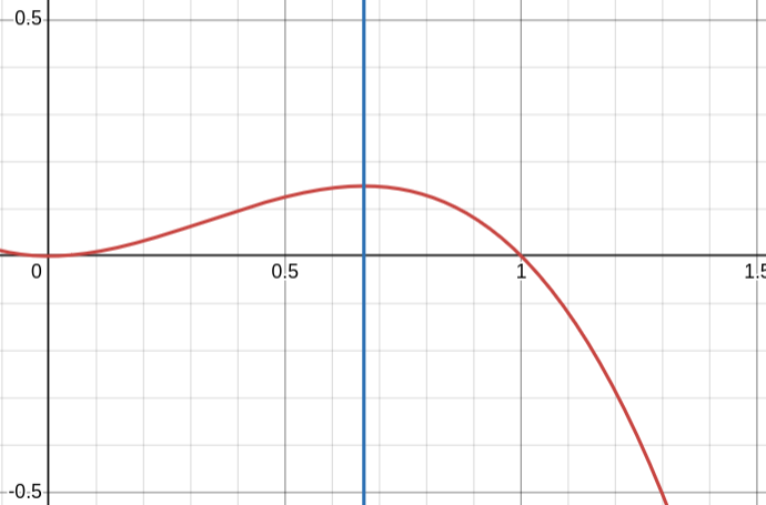
So, since the chance to get heads is not $50\%$ we conclude that the coin is unfair.
You can notice that all that math is a bit of an overkill, since we could have just counted the frequencies and get the same answer. Meaning, there were 3 tosses, 2 of which were heads, so we could say that the probability of getting heads is $\frac{2}{3}$, so coin is unfair. But I wanted to present MLE as an optimization problem, since that’s the way of thinking I enjoy and that is what going to lead us to the factor graph optimization.
Of course, MLE is naive. Coin could be fair, and we just happened to get two heads in a row. To fix this, we need to consider a prior knowledge given to us in the problem. That’s where the actual Bayes inference is used.
Maximum a Posteriori
The second approach, is Maximum a Posteriori (MAP) method. This one actually utilizes the Bayes rule. By the way, here’s the rule itself:
In our problem, the hypothesis $H$ is our estimate of $\theta$, the experiment $E$ is the observed data, and in MAP estimation our goal is to maximize the posterior distribution $P(H|E)$. Now, let’s get all of the pieces together.
The probability of the coin landing heads $N_h$ times and tails $N_t$ times (experiment $E$) given probability of the coin landing heads $\theta$ (hypothesis) is a Binomial distribution. So, in our case:
\[P(E|H) = P(\text{"observed data"} | \theta) = \theta^{N_h}(1-\theta)^{N_t}\]The probability of the hypothesis $P(H)$ represents our prior belief about $\theta$ (fairness of the coin). When dealing with Binomial distributions, it’s common to choose Beta distribution as a prior. Beta distribution, essentially, represents “virtual” MLE with two parameters: $\alpha$ - the number of virtual successes and $\beta$ - the number of virtual failures. For example, if we want to represent a prior belief that the coin is fair, we might choose $\alpha=50$ and $\beta=50$, i.e. we’ve observed equally many successes and failures. If we believe that the coin is more likely to land tails, we might choose $\alpha=10$ and $\beta=50$. I hope the idea is clear. So, our prior belief is modeled as:
\[P(H) = \theta^{\alpha - 1}(1-\theta)^{\beta-1}\]The great thing about the MAP is that we can ignore the denominator $P(E)$, since we’re trying to find $\theta$, that maximizes $P(\theta|E)$ and $P(E)$ does not depend on $\theta$. Therefore, we build our cost function:
\[\mathcal{L}(\theta) = P(\theta|E) = \frac{P(E|\theta) \cdot P(\theta)} {P(E)} \propto P(E|\theta) \cdot P(\theta) = \\ \theta^{N_h}(1-\theta)^{N_t} \cdot \theta^{\alpha - 1}(1-\theta)^{\beta-1} = \theta^{N_h + \alpha - 1}(1-\theta)^{N_t + \beta - 1}\]Now, let’s say our observations are the same as before: $\vec{x_o} = [x_1, x_2, x_3] = [1, 1, 0]$ and the friend we trust ensured us the coin was fair. Then we choose $\alpha=10$ and $\beta=10$ and rewrite:
\[\mathcal{L} = \theta^{2 + 10 - 1}(1-\theta)^{1 + 10 - 1} = \theta^{11}(1-\theta)^{10}\]The plot looks very flat on $[0,1]$, but $\theta_{max} = 0.523 \approx \frac{1}{2}$ - maximizes $\mathcal{L}$. Notice how this time, in contrast to the MLE, the fact that 2 out of 3 tosses were heads was overweighted by our strong prior belief and we conclude that the coin is fair.
Conclusions
In this article I talked about two common approaches to probabilistic inference - MLE and MAP. While not too complicated, those two approaches are fundamental and serve as a basis for many others. I talked about the basic coin fairness problem for simplicity. In the next part of the series I’ll introduce a more complicated problem - 2D localization. I’ll discuss how to use MAP to solve it, and what are the problems that one would encounter.